I stumbled across this fascinating YouTube video about how Shazam works and was immediately hooked. The technology behind recognizing songs from short audio clips was so interesting I had to dive deeper. You can’t tell me you don’t have intense urges to understand random topics in their entirety.
No? Just me? Whatever.
When I was researching this topic taking a bunch of notes a grand and completely unique idea came to mind. Why not blog about it! Almost as bad as starting a podcast man where have my morals gone. Whatever now I get to freely rant or teach random topics to the void. Making my mark on the interwebs.
Allow me to attempt and break down the science behind the algorithms powering Shazam in a way that’s hopefully both understandable and accurate :)
Music and Physics
Lets start with the basics, a sound is a vibration that propagates through air (or water) and can be decrypted by ears.
In the same manner light is also a vibration, you can’t hear it because your ears cant decrypt it, but your eyes can.
Pure Tones Vs Real Sounds
A pure tone is a tone with a sinusodial waveform (fancy way of saying sine wave) which as a reminder is the most natural representation of how many things in nature change state. Remember a sine wave is characterized by:
- Frequency: Number of cycles per second. Its unit is Hertz (Hz), 100Hz = 100 cycles per second
- Amplitude (related to loudness of sound): The size of each cycle
These characteristics are decrypted by the ear to form a sound. Humans can hear pure tones from 20 Hz to 20,000 Hz!!! What a range unfortunately that range does decrease as we age :(
By comparison the light we see is composed of sinewaves from 4 x 10^14 Hz to 7.9 x 10^14 Hz
The human perception of loudness depends on the frequency of the pure tone. For instance, a pure tone at an amplitude 10 with a frequency of 30Hz will be quieter than a pure tone with an amplitude 10 of frequency 1000Hz. Human ears follow the psychoacoustic model.
Pure tones dont naturally exist but every sound in the world is the sum of a multiple pure tones at different amplitudes. We’ll get into this later.
Musical Notes
A music partition is a set of notes executed at a certain moment. These notes also have a duration and a loudness.
The notes are divided in octaves, a set of 8 notes.
- The frequency of a note in an octave doubles in the next octave. For example, the frequency of A4 (A in the 4th octave) at 440Hz equals 2 times the frequency of A3 (A in the 3rd octave) at 220Hz and 4 times the frequency of A2 (A in the 2nd octave) at 110Hz.
Many instruments provides more than 8 notes by octaves, those notes are called semitone or halfstep.
For the 4th octave the notes have the following frequency:
- C4 (or Do3) = 261.63Hz
- D4 (or Re3) = 293.67Hz
- E4 (or Mi3) = 329.63Hz
- F4 (or Fa3) = 349.23Hz
- G4 (or Sol3) = 392Hz
- A4 (or La3) = 440Hz
- B4 (or Si3) = 493.88Hz
The frequency of the sensitivity of our ears is logarithmic. This means that:
- between 32.70 Hz and 61.74Hz lies the 1st octave
- between 261.63Hz and 466.16Hz lies the 4th octave
- between 2 093 Hz and 3 951.07Hz lies the 7th octave
- and so on…
Human ears will be able to detect the same number of notes.
The A4 (or La3) at 440Hz is a standard reference for the calibration of acoustic equipment and musical instruments.
Timbre
You may notice that the same note doesn’t sound exactly the same if its played by a guitar, a piano, a violin, or a human singer. The reason is that each instrument has its own timbre for a given note.
For each instrument, the sound produced is a multitude of frequencies that sound like a given note (the scientific term for a musical note is a pitch). This sound has a fundamental frequency (the lowest frequency) and multiple overtones (any frequency higher than the fundamental).
Most instruments produce ( close to) harmonic sounds. For those instruments, the overtones are multiples of the fundamental frequency called harmonics.
For example the composition of pure tones A2 (fundamental), A4 and A6 is harmonic whereas the composition of pure tones A2, B3, F5 is inharmonic.
Many percussion instruments ( like cymbals or drums) create inharmonic sounds.
Spectrogram
A music song is played by multiple instruments and singers. All those instruments produce a combination of sinewaves at multiple frequencies and the overall is an even bigger combination of sinewaves.
It is possible to see music with a spectrogram. Most of the time, a spectogram is a 3 dimensional graph where:
- the X-axis represents time
- the Y-axis represents the frequency of the pure tone
- the Z-axis or the third dimension is described by a color and it represents the amplitude of a frequency at a certain time
An interesting fact is that the intensity of the frequencies changes through time. it’s another particularly of an instrument that makes it unique. If you take the same artist but you replace the piano, the evolution of the frequencies won’t behave the same and the resulting sound will be slightly different because each artist/instrument has its own style. Technically speaking, these evolutions of frequencies are modifying the envelope of the sound signal.
Digitalization
Unless you’re a vinyl disk lover, when you listen to music you’re using a digital file (mp3, apple lossless, ogg, audio CD, whatever) but when artists produce music, it is analogical (not represented by bits). This music is digitized in order to be stored and played by electronic devices.
Sampling
Analog signals are continuous signals, which means if you take one second of an analog signal, you can divide this second into (put the greatest number you can think of and I hope it’s a big one) parts that last a fraction of a second. In the digital world, you can’t afford to store an infinite amount of information. You need to have a minimum unit, for example 1 millisecond. During this unit of time the sound cannot change so this unit needs to eb short enough so that the digital song sounds like the analog one and big enough to limit the space needed for storing the music.
For example, think about your favorite music. Now think about it with the sound changing only every 2 seconds, it sounds like nothing. Tehcnically speaking the sound is aliased. In order to be sure that your song sounds great you can choose a very small unit like a nano (10^-9) second. This tiem your music sounds great but you don’t have enough disk space to store it, welp that’s too bad.
This problem is called sampling.
The standard unit of time in digital music is 44,100 units (or samples) per second.
Where does this 44.1kHz come from?
Humans can hear sounds from 20Hz to 20kHz, a theorem from Nyquist and Shannon states that if you want to digitize a signal from 0Hz to 20kHz you need at least 40,000 samples per second. The main idea is that a sine wave signal at a frequency F needs at least 2 points per cycle to be identified. If the frequency of your sampling is at least twice the frequency of your signal, you’ll end up with at least 2 points per cycle of the original signal.
Lets put together an image in python:
import numpy as np
import matplotlib.pyplot as plt

# Define parameters
f = 20  # frequency of the sine wave in Hz
t_start = 0
t_end = 0.16
sampling_rate = 40  # sampling rate in Hz

# Calculate phase shift so that y(0) = -0.6
phi = np.arcsin(-0.6)

# Create a high resolution time vector for the continuous wave
t_cont = np.linspace(t_start, t_end, 1000)
y_cont = np.sin(2 * np.pi * f * t_cont + phi)

# Create the sampling time vector
t_sample = np.arange(t_start, t_end + 1/sampling_rate, 1/sampling_rate)
y_sample = np.sin(2 * np.pi * f * t_sample + phi)

# Create the plot
plt.figure(figsize=(8, 4))

# Plot continuous wave as blue curve
plt.plot(t_cont, y_cont, 'b-', label='20Hz Continuous Wave')

# Plot the sampled points connected by a green line
plt.plot(t_sample, y_sample, 'g-', label='40Hz Sampled Line')

# Plot the sampled points as red crosses
plt.plot(t_sample, y_sample, 'rx', markersize=8, label='Sampled Points')

# Labeling the axes and adding title and legend
plt.xlabel('Time (seconds)')
plt.ylabel('Amplitude')
plt.title('20Hz Sine Wave Sampled at 40Hz with Phase Shift')
plt.legend()
plt.grid(True)
plt.tight_layout()

# Display the plot
plt.show()
The resulting image is
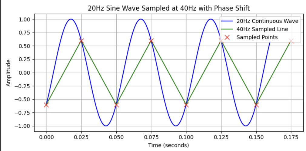
A sound at 20Hz is digitalized using a 40Hz sampling rate:
- the blue curve represents the sound at 20Hz
- the red crosses represent the sampled sound, which means I marked the blue curve with a red cross every 1/40 second
- the green line is an interpolation of the sample sound
Though it hasn’t the same shape nor the same amplitude, the frequency of the sampled signal remains the same.
Now lets code together a bad example, with the same 20Hz sound being digitalized by a 30Hz sampling rate:
import numpy as np
import matplotlib.pyplot as plt

# Define parameters
f = 20  # frequency of the sine wave in Hz
t_start = 0
t_end = 0.16
sampling_rate = 30  # sampling rate in Hz

# Calculate phase shift so that y(0) = -0.6
phi = np.arcsin(-0.6)

# Create a high resolution time vector for the continuous wave
t_cont = np.linspace(t_start, t_end, 1000)
y_cont = np.sin(2 * np.pi * f * t_cont + phi)

# Create the sampling time vector
t_sample = np.arange(t_start, t_end + 1/sampling_rate, 1/sampling_rate)
y_sample = np.sin(2 * np.pi * f * t_sample + phi)

# Create the plot
plt.figure(figsize=(8, 4))

# Plot continuous wave as blue curve
plt.plot(t_cont, y_cont, 'b-', label='20Hz Continuous Wave')

# Plot the sampled points connected by a green line
plt.plot(t_sample, y_sample, 'g-', label='30Hz Sampled Line')

# Plot the sampled points as red crosses
plt.plot(t_sample, y_sample, 'rx', markersize=8, label='Sampled Points')

# Labeling the axes and adding title and legend
plt.xlabel('Time (seconds)')
plt.ylabel('Amplitude')
plt.title('20Hz Sine Wave Sampled at 40Hz with Phase Shift')
plt.legend()
plt.grid(True)
plt.tight_layout()

# Display the plot
plt.show()
The output would be:
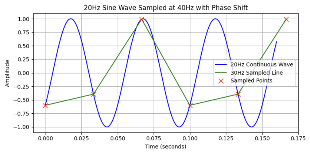
We can see a sound at 20 Hz being digitalized with a 30Hz sampling rate. The frequency of the sampled signal is not the same as the original signal: it’s only 10Hz. If you look carefully, you can see that one cycle in the sampled signal represents two cycles in the original signal. This case is an under sampling.
If you want to digitize a signal between 0Hz and 20kHz, you need to remove from the signal its frequencies over 20kHz before the sampling. Otherwise those frequencies will be transformed into frequencies between 0Hz and 20kHz and therefore add unwanted sounds (called aliasing).
If you want a good music conversion from analogic to digital you have to record the analog music at least 40,000 times per second. HIFI corporations (like Sony) chose 44,1kHz during the 80s because it was above 40,000Hz and compatible with the video norms NTSC and PAL. Other standards exist for audio like 48 kHz (Bluray), 96 kHz or 192 kHz but if you’re neither a professional nor an audiophile you’re likely to listen to 44.1 kHz music.
More on Nyquist-Shannon sampling theorem here. The frequency of the sampling rate needs to be strictly superior of 2 times the frequency of the signal to digitize because if the worst case scenerio, you could end up with a constant digitalized signal.
Quantization
We know how to digitize the frequencies of analogic music, but what about its loudness? The loudness is a relative measure: the same loudness inside the signal, if you increase your speakers the sound will be higher. The loudness measures the variation between the lowest and the highest level of sound inside a song.
The same problem as before, how to pass from a continuous world (an infinite variation of volume) to a discrete one?
Imagine your favorite music with only 4 states of loudness: no sound, low sound, high sound and full power. Even the best song in the world becomes unbearable. What you’ve just imagined was a 4-level quantization.
Lets code an example of a low quantization of an audio signal.
import numpy as np

import matplotlib.pyplot as plt


# Parameters

fs = 44100 # Sample rate (Hz)

duration = 0.012 # 12 milliseconds

t = np.linspace(0, duration, int(fs * duration), endpoint=False) # Time array


# Generate a sample audio signal (a mix of sinusoids)

audio_signal = 8 * np.sin(2 * np.pi * 110 * t) + 2 * np.sin(4 * np.pi * 210 * t)


# 8-level quantization

# Define 8 levels between -10 and 10

levels = np.linspace(-10, 10, 8)

# Find the nearest level for each sample

quantized_signal = np.zeros_like(audio_signal)

for i, sample in enumerate(audio_signal):a

idx = np.abs(levels - sample).argmin()

quantized_signal[i] = levels[idx]


# Create the plot

plt.figure(figsize=(10, 6))

plt.plot(t, audio_signal, 'b-', linewidth=1.5, label='Original Signal')

plt.plot(t, quantized_signal, 'r-', linewidth=1, label='8-level Quantized')

plt.axhline(y=0, color='k', linestyle='-', alpha=0.3)

plt.grid(True, alpha=0.3)


# Set plot parameters

plt.xlim(0, duration)

plt.ylim(-10, 10)

plt.xlabel('Time (seconds)')

plt.ylabel('Amplitude')

plt.title('Audio Signal and 8-level Quantization')

plt.legend()


# Add horizontal lines for the quantization levels

for level in levels:

plt.axhline(y=level, color='gray', linestyle='--', alpha=0.4)


plt.tight_layout()

plt.show()
The resulting image:
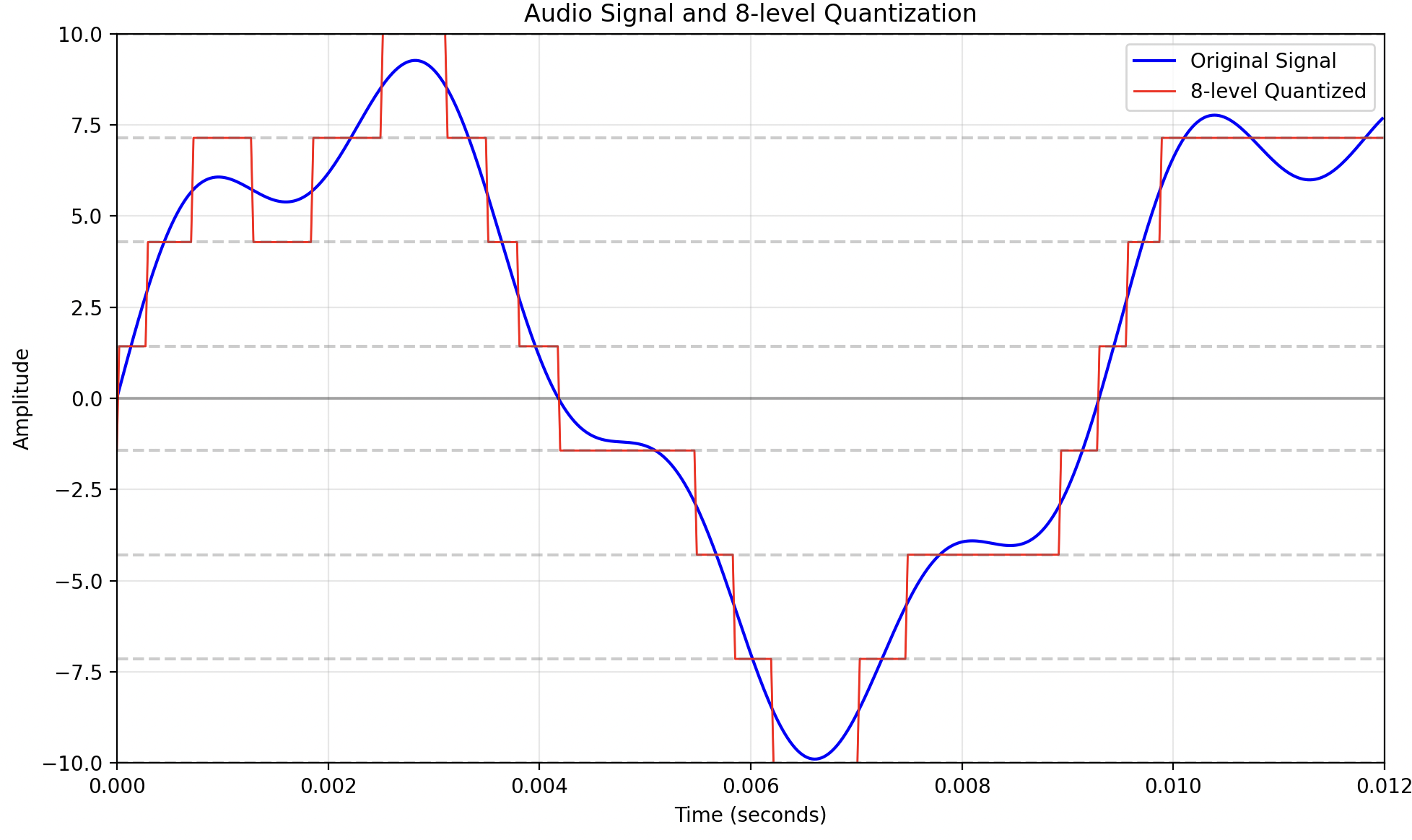
This represents an 8 level quantization. As we can see the resulting sound (in red) is called quantization error or quantization noise. This 8 level quantization is also called a 3 bits quantization because you only need 3 bits to implement the 8 different levels (8 = 2^3).
Here is the same signal with a 64 levels quantization (or 6 bits):
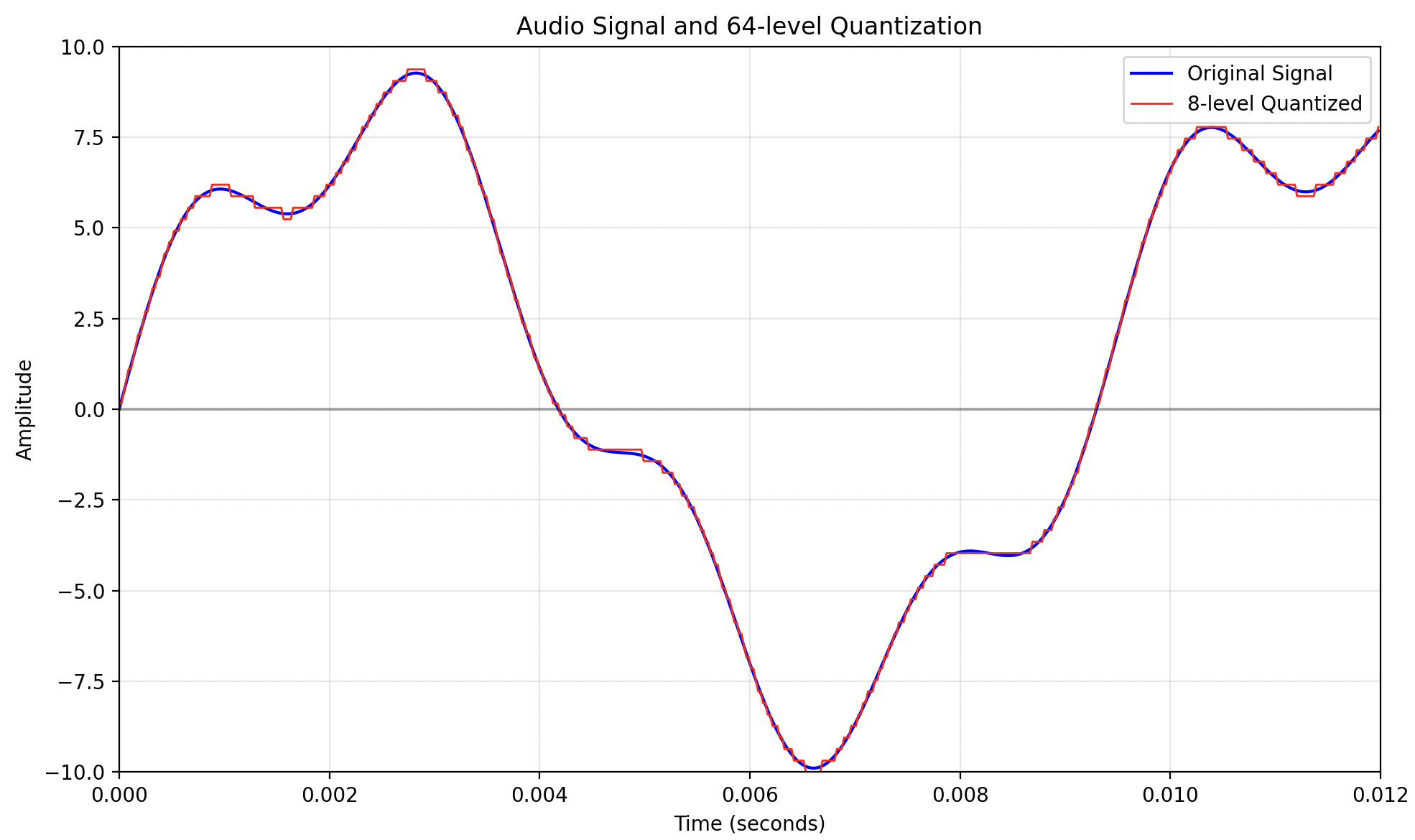
Though the resulting sound is still altered, it looks (and sounds) a lot more like the original sound.
Thankfully we dont have extra sensitive ears. The standard quantization is coded on 16 bits, which means 65,536 levels. With a 16 bitz quantization, the quantization noise is low enough for human ears.
In studio, the quantization used by professionals is 24 bits, which means there are 2^24(16 million) possible variations of loudness between the lowest point of the track and the highest. I made some approximations in my examples concerning the number of quantization levels.